Simple nonlinear least squares curve fitting in Python

The problem

Today we are going to test a very simple example of nonlinear least squares curve fitting using the scipy.optimize module.

%matplotlib inline
import numpy as np
import matplotlib.pyplot as plt
from scipy.optimize import curve_fit

Create data

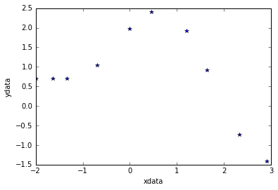
Let’s assume we have the following points [xdata, ydata] and that we want to fit these data with the following model function using nonlinear least squares:

$F(p_1,p_2,x) = p_1\cos(p_2x) + p_2\sin(p_1x)$

For now, we are primarily interested in the following results:

• The fit parameters
• Sum of squared residuals

xdata = np.array([-2,-1.64,-1.33,-0.7,0,0.45,1.2,1.64,2.32,2.9])
ydata = np.array([0.699369,0.700462,0.695354,1.03905,1.97389,2.41143,1.91091,0.919576,-0.730975,-1.42001])

# Show data points
plt.plot(xdata,ydata,'*')
plt.xlabel('xdata')
plt.ylabel('ydata');

Define fit function

def func(x, p1,p2):
  return p1*np.cos(p2*x) + p2*np.sin(p1*x)

Calculate and show fit parameters.

Use a starting guess of $p_1=1$ and $p_2=0.2$

The outputs of the curve_fit function are the following:

• popt : array of optimal values for the parameters so that the sum of the squared error of $f(xdata, *popt) - ydata$ is minimized

• pcov : 2d array of the estimated covariance of popt. The diagonals provide the variance of the parameter estimate. To compute one standard deviation errors on the parameters use $perr = np.sqrt(np.diag(pcov))$. If the Jacobian matrix at the solution doesn’t have a full rank, then ‘lm’ method returns a matrix filled with np.inf, on the other hand ‘trf’ and ‘dogbox’ methods use Moore-Penrose pseudoinverse to compute the covariance matrix.

popt, pcov = curve_fit(func, xdata, ydata,p0=(1.0,0.2))

print("Parameter estimation results:")
print("p1 = ",popt[0]," | p2 = ",popt[1])
print("--------------------------")
print("Covariance matrix of the estimate:")
print(pcov)

Parameter estimation results:
p1 =  1.881850994  | p2 =  0.700229857403
--------------------------
Covariance matrix of the estimate:
[[  7.52408290e-04   1.00812823e-04]
 [  1.00812823e-04   8.37695698e-05]]

Sum of squares of residuals

Since it’s not given by the curve_fit function, we have to compute it by hand

p1 = popt[0]
p2 = popt[1]
residuals = ydata - func(xdata,p1,p2)
fres = sum(residuals**2)

print("Residuals sum of squares:")
print(fres)

Residuals sum of squared:
0.0538126964188

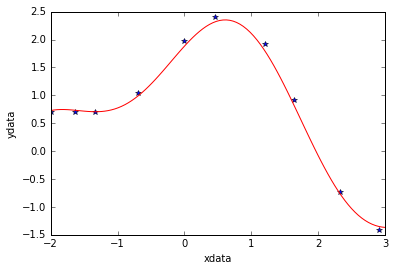
Plot fitted curve along with data

curvex=np.linspace(-2,3,100)
curvey=func(curvex,p1,p2)
plt.plot(xdata,ydata,'*')
plt.plot(curvex,curvey,'r')
plt.xlabel('xdata')
plt.ylabel('ydata');